Mastering Data Visualization: Excel’s PieChart Master Tool Comprehensive Guide
Data visualization is a key aspect of data management that enables stakeholders to understand and interpret data quickly and effectively through visual representations. Among various data visualization tools, Excel’s PieChart feature stands as a versatile and powerful method to display proportions and relationships within datasets. This comprehensive guide aims to break down the complexities of PieCharts in Excel, making them accessible and useful for both beginners and advanced users.
**What are PieCharts?**
PieCharts provide a visual breakdown of data into distinct segments. Each segment, or slice of the pie, represents a portion of the whole, making it easy to identify the relative size of each component. Ideal for showing data distribution, budget allocations, market shares, or any scenario where comparison of parts versus the whole is crucial.
**Creating a PieChart in Excel**
1. **Data Preparation**: Start by organizing your data in a table format with categories in one column and values in another.
2. **Select Your Data**: Highlight the data range you wish to represent in the PieChart. Be sure to include the category labels.
3. **Navigate to the Chart Section**: Click on the “Insert” tab in the Excel ribbon, then select the “Insert Chart” icon. From there, choose “Pie” from the chart types available. Various subtypes such as 2D pie, 3D pie, and doughnut charts offer varying perspectives for your information.
4. **Personalize Your Chart**:
– **Title**: Add a descriptive title at the top of your chart to give it immediate context.
– **Legend**: Customize the legend to ensure it is detailed enough to identify each segment clearly. This is particularly useful in charts with many segments.
– **Slices**: Adjust the size of slices for clarity by right-clicking and selecting “Add Data Labels” or “Format Data Series” options. Toggle labels between percentage and value formats as needed.
– **Design and Layout**: Customize the appearance of your chart elements, adjusting colors, fonts, and the overall style to align with your presentation standards or organization’s branding.
**Advanced Techniques**
– **Exploring Doughnut Charts**: Similar to PieCharts, Doughnut charts offer a unique visual distinction with a hollow center, allowing multiple circles to be displayed. They are ideal for comparing components across groups.
– **Exploding Slices**: Emphasize specific data points by “exploding” or separating a slice from the chart. This technique can highlight individual categories and make them stand out for a more impactful visual presentation.
– **Slice Transparency**: Adjusting the transparency of slices can be particularly effective when displaying large data volumes, helping to avoid clutter and making comparisons easier between many segments.
**Chart and Data Compatibility**:
– **Updating Charts with Live Data**: Excel allows for dynamic updating of charts based on changes made to the data. Ensure data ranges are referenced correctly to avoid inconsistencies.
– **Conditional Formatting**: Enhance the informational value of your PieCharts by applying conditional formatting to slices based on their position or value. This adds an extra layer of analysis, enabling readers to understand not just the absolute values but also trends or thresholds achieved within your data.
**Conclusion**
Mastering Excel’s PieChart functionality enables you to effectively communicate complex data relationships, making it an incredibly useful tool for both professional reports and educational materials. Remember, the true power of a PieChart lies in how effectively it presents information. By following these guidelines and incorporating advanced techniques, you can take your data visualization skills to the next level, ensuring that your data insights are not only accurate but also engaging and impactful to diverse audiences.

